Camera Calibration Demystified: Part 1 - Fundamentals and Models
Introduction
Imagine you're taking a photo of a building with your smartphone. You might notice that the lines of the building don't appear as straight as they do in real life, or the proportions seem slightly off. These are distortions, and discrepancies between the real-world objects and their representations in the image. Such distortions often occur due to the inherent limitations of camera lenses and sensors as they attempt to map a 3D world onto a 2D plane.
Camera calibration is the technique used to understand and correct these distortions. It's a fundamental process for achieving more accurate visual representations, especially in applications like augmented reality, robotics, and 3D reconstruction. In this first part of our series on camera calibration, we'll explore the foundational concepts and models that serve as the backbone of this technique. We'll delve into the intrinsic and extrinsic parameters that influence how a camera captures an image and discuss how these parameters can be determined to correct distortions. By the end of this post, you'll have a solid understanding of the principles behind camera calibration and its importance in various domains.
Camera Models
To understand the intricacies of camera imaging, it's useful to connect the dots with real-world applications. Take the example of a self-driving car, which relies on its camera to accurately gauge the dimensions and distances of surrounding elements like pedestrians, other vehicles, and road signs. Just as understanding the human eye's perception aids in comprehending our interaction with the 3D world, grasping the mechanics of a camera model enhances the precision of such measurements in automated systems. To unpack this further, let's engage in a thought experiment: envision a simple setup (See figure 1) where a small barrier with a pinhole is placed between a 3D object and a film. Light rays from the object pass through the pinhole to create an image on the film. This basic mechanism serves as the cornerstone for what is known as the pinhole camera model, a foundational concept that allows us to fine-tune the way cameras, like the one in a self-driving car, interpret the world.
Pinhole Camera Model
The setup
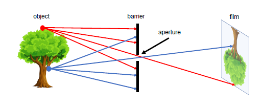
In the pinhole model, consider a 3D coordinate system defined by unit vectors i, j, k. Place an object point P with coordinates (X, Y, Z) in this world. The camera's aperture is at the origin O, and the image plane (or film) is parallel to the i-j plane at a distance f along the k-axis. The film has a centre C', and the projection of P onto the film is P' with 2D coordinates (x, y) - (Refer to Figure 1 and 2)
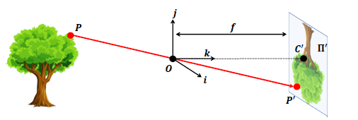
The Mathematics
To relate P and P', we draw a line from P through the aperture O, intersecting the film at P'. The triangles POP' and OCP' are similar, which gives us:
$$\frac{x}{f} = \frac{X}{Z} \quad \text{and} \quad \frac{y}{f} = \frac{Y}{Z}$$
Solving for x and y, we get:
$$\begin{align*} x &= f \left( \frac{X}{Z} \right), \\ y &= f \left( \frac{Y}{Z} \right). \end{align*}$$
Here, f represents the focal length of the Camera.
Lens Models
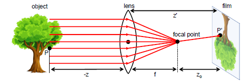
While the pinhole model gives us an idealized perspective of image formation, real-world cameras use lenses to focus light. Lenses introduce additional complexities due to their shape, material, and how they bend light rays. These models account for additional factors like focal length, aperture, and lens distortions. Let's explore lens models to understand these intricacies.
The Setup
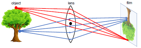
Like the pinhole model, lens models use a 3D coordinate system defined by i, j, k. However, instead of a pinhole at O, we have a lens. The image plane is still at a distance f along the k-axis, we denote the centre of this plane as C' (Refer to Figure 3 and 4)
The Mathematics
In lens models, we need to account for distortions introduced by the lens. These distortions are typically represented by dx and dy, affecting the x and y coordinates, respectively. The equations for x and y in lens models are:
$$\begin{align*} x &= f \left( \frac{X}{Z} \right) + d_x, \\ y &= f \left( \frac{Y}{Z} \right) + d_y. \end{align*}$$
In these equations, dx and dy are functions of X, Y, and Z and they represent the distortions introduced by the lens.
Intrinsic and Extrinsic Parameters
So far, we've discussed the basic models that describe how cameras work and how they capture the 3D world onto a 2D plane. These models give us a high-level view but are generalized and often idealized. In practice, each camera has its unique characteristics that influence how it captures an image. These characteristics are captured by what are known as intrinsic and extrinsic parameters. While intrinsic parameters deal with the camera's own 'personality' or 'DNA' extrinsic parameters describe how the camera is positioned in space. Together, they offer a complete picture of a camera's behaviour, which is crucial for applications like 3D reconstruction, augmented reality, and robotics.
Intrinsic Parameters
After Understanding the broad overview of intrinsic and extrinsic parameters, let's zoom in on the intrinsic parameters first. These parameters are unique to each camera and provide insights into how it captures images. While these parameters are generally considered constants for a specific camera, it is important to note that they can sometimes change. For instance, in cameras with variable focal lengths or adjustable sensors, intrinsic parameters can vary.
Optical Axis
The optical axis is essentially the line along which light travels into the camera to hit the sensor. In the idealized pinhole and lens models, it's the line that passes through the aperture (or lens centre) and intersects the image plane. It serves as a reference line for other measurements and parameters.
Focal Length (f ): This is the distance between the lens and the image sensor. Knowing the focal length is crucial for estimating the distances and sizes of objects in images. It's also a key factor in determining the field of view and is usually represented in pixels.
$$f = \alpha \times \text{sensor size} ,$$
$$\text{Here}, \alpha \space \text{is a constant that relates the physical sensor size to the size in pixels}$$
- Principal Point ((cx, cy)): This is the point on the image plane where the optical axis intersects, it often lies near the centre of the image. it is crucial for tasks like image alignment and panorama stitching.
$$\begin{align*} c_x &= \frac{Image Width}{2},\\ \\ c_y &= \frac{Image Height}{2}. \end{align*}$$
- Skew Coefficient (s): This parameter is responsible for any angle between the x and y pixel axes of the image plane. It is rarely encountered in modern-day cameras.
$$s = 0 \quad \text{(usually)}$$
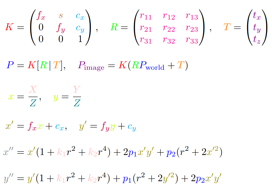
The intrinsic matrix denoted by K consolidates these parameters:
$$K = \begin{pmatrix} f_x & s & c_x \\ 0 & f_y & c_y \\ 0 & 0 & 1 \end{pmatrix}$$
Note on Constancy
Although intrinsic parameters like the focal length and principal point are often treated as constants, especially in fixed or pre-calibrated camera setups, they can often change based on specific hardware configurations. For example, the focal length will vary in cameras with zoom capabilities. Therefore, in such special cases, recalibration may be necessary.
Camera with Zoom Capabilities
Cameras with zoom capabilities introduce an additional layer of complexity to the calibration process. While Zooming allows for better framing or focus on specific areas, it also changes intrinsic parameters like the focal length. This section will explore how to handle calibration in scenarios involving zoom.
Calibration at Specific Zoom Levels
When you calibrate a camera at a particular zoom level, the resulting intrinsic parameters are only accurate for that setting. If you continue to record or capture images at the same zoom level, these calibration parameters will remain valid.
$$K_{\text{zoom}} = \begin{pmatrix} f_{\text{zoom}} & s & c_x \\ 0 & f_{\text{zoom}} & c_y \\ 0 & 0 & 1 \end{pmatrix}$$
Here, Kzoom and fzoom represent the camera matrix and focal length at the specific zoom level, respectively.
Handling Zoom Changes
If you adjust the zoom after calibration, you have two main options:
Dynamic Calibration: Recalibrate the camera every time you change the zoom. This approach provides the highest accuracy but may be impractical for real-time applications due to computational costs.
.Parameter Interpolation: If you've calibrated the camera at multiple zoom levels, you can interpolate the intrinsic parameters for new zoom settings. This is computationally efficient but might sacrifice some accuracy.
Understanding intrinsic parameters is key for various computer vision tasks. For instance, in augmented reality, an accurate intrinsic matrix can drastically improve the realism and alignment of virtual objects in real-world scenes.
Extrinsic Parameters
While intrinsic parameters define a camera's 'personality' by capturing its internal characteristics, extrinsic parameters tell the 'story' of the camera's interaction with the external world. These parameters, specifically the rotation matrix R and the translation vector T, are indispensable for mapping points from the camera's 2D image plane back to their original 3D coordinates in the world. This becomes particularly vital in scenarios involving multiple cameras or moving cameras, such as in robotics or autonomous vehicles. By accurately determining these extrinsic parameters, one can achieve high-precision tasks like 3D reconstruction and multi-camera scene analysis.
Rotation Matrix (R): This 3x3 matrix gives us the orientation of the camera in the world coordinate system. Specifically, it transforms coordinates from the world frame to the camera frame. For instance, if a drone equipped with a camera needs to align itself to capture a specific scene, the rotation matrix helps in determining the orientation the drone must assume.
The rotation matrix is usually denoted as R and takes the form:
$$R = \begin{pmatrix} r_{11} & r_{12} & r_{13} \\ r_{21} & r_{22} & r_{23} \\ r_{31} & r_{32} & r_{33} \end{pmatrix}$$
The elements r11, r12, and r13, .... r33 define the camera's orientation relative to the world's coordinate system. Each column of R essentially represents the unit vectors along the camera's local x, y, and z axes, but expressed in terms of the world coordinate system. For example, r11, r21, and r31 describe how much the world's x-component aligns with the camera's local x-axis.
- Translation Vector (T): This 3x1 vector represents the position of the camera's optical centre in the world coordinate system. The translation vector is generally represented as:
$$T = \begin{pmatrix} t_x \\ t_y \\ t_z \end{pmatrix}$$
The elements tx, ty, and tz in the translation vector represents the position of the camera's optical centre in the world coordinate system. For instance, tx is the distance from the world origin to the camera's optical centre along the world's x-axis, while ty and tz serve the same purpose along the y and z axes, respectively.
Computing R and T gives you a complete picture of the camera's pose in the world, including both orientation and position.
Together, the rotation matrix and the translation vector can be combined into a single 3x4 matrix, often represented as [R|T]:
$$[R|T] = \begin{pmatrix} r_{11} & r_{12} & r_{13} & t_x \\ r_{21} & r_{22} & r_{23} & t_y \\ r_{31} & r_{32} & r_{33} & t_z \end{pmatrix}$$
Conclusion
We've covered a lot of ground in this first instalment of our series on camera calibration, unravelling the complexities behind camera models and the intrinsic and extrinsic parameters that define them. These foundational concepts are the building blocks for more advanced topics like distortion correction, 3D reconstruction, and multi-camera setups. In the next part of this series, we'll go beyond the basics to explore the practical reasons for camera calibration, the types of distortions you might encounter, and the mathematical and technical approaches to correct them. So, stay tuned for more insights into the fascinating world of camera calibration!
References
For those looking to delve deeper into the topics covered in this blog post, the following resources are highly recommended:
[1] Multiple View Geometry in Computer Vision by Richard Hartley and Andrew Zisserman
[2] Stanford CS231A: Camera Models
Further Reading
For those looking to delve deeper into the topics covered in this blog post, the following resources are highly recommended:
Books:
Digital Image Warping by George Wolberg
Multiple View Geometry in Computer Vision by Richard Hartley and Andrew Zisserman
Computer Vision: Algorithms and Applications by Richard Szeliski
3D Computer Vision: Efficient Methods and Applications by Christian Wöhler
Papers:
A Four-step Camera Calibration Procedure with Implicit Image Correction by Jean-Yves Bouguet
Flexible Camera Calibration By Viewing a Plane From Unknown Orientations by Zhengyou Zhang
By exploring these resources, you'll gain a more comprehensive understanding of camera calibration, enabling you to tackle more complex problems and applications.